Tutorial
In this tutorial, we will give a brief introduction on the quantization and pruning techniques upon which QSPARSE is built. Using our library, we guide you through the building of a image classification neural network with channel pruning and both weights and activations quantized.
If you are already familiar with quantization and pruning methods and want to learn the programming syntax, please fast forward to Building Network with QSPARSE.
Preliminaries
Quantization and pruning are core techniques used to reduce the inference costs of deep neural networks and have been studied extensively.
Quantization
Approaches to quantization are often divided into two categories:
- Post-training quantization
- Quantization aware training
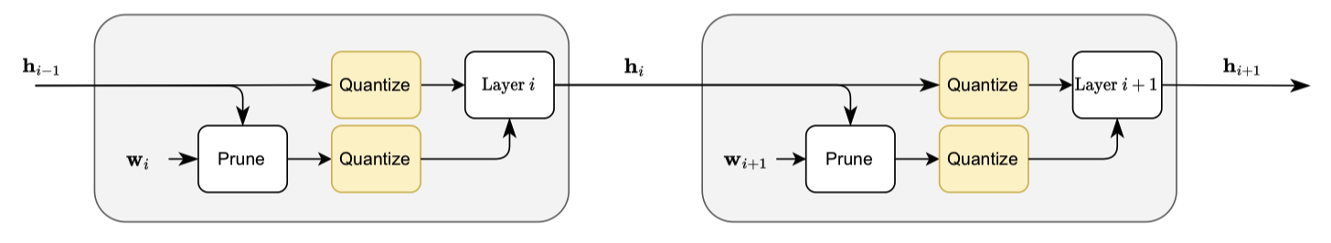
The former applies quantization after a network has been trained, and the latter quantizes the network during training and thereby reduces the quantization error throughout training process and usually yields superior performance. Here, we focus on quantization aware training by injecting quantization operator into the training computational graph. Our quantization operator implements a variant of STE-based uniform quantization algorithm introduced in our MDPI publication.
Pruning
Magnitude-based pruning is often considered one of the best practice to produce sparse network during training. Through using activation or weight magnitude as a proxy of importance, neurons or channels with smaller magnitude are removed. In practice, the element removal is accomplished by resetting them to zero through multiplication with a binary mask. The elmement removal and magnitude estimation are done by the pruning operator injected in the computational graph. Our pruning operator supports unstructured and structured pruning, and can be targeted to support layerwise pruning, as proposed in our MDPI publication, and stepwise pruning as proposed by Zhu et al..
Building Network with QSPARSE
With the above methods in mind, in the following, we will use QSPARSE to build a quantized and sparse network upon the below full precision network borrowed from pytorch official MNIST example.
%load_ext autoreload
%autoreload 2
import numpy as np
import torch
import torch.nn as nn
import torch.nn.functional as F

class Net(nn.Module):
    def __init__(self):
        super(Net, self).__init__()
        self.conv_part = nn.Sequential(
            nn.Conv2d(1, 32, 3, 1),
            nn.BatchNorm2d(32),
            nn.ReLU(),
            nn.Conv2d(32, 64, 3, 1),
            nn.BatchNorm2d(64),
            nn.ReLU(),
            nn.MaxPool2d(2),
            nn.Dropout(0.25),

        )
        self.linear_part = nn.Sequential(
            nn.Flatten(),
            nn.Linear(9216, 128),
            nn.BatchNorm1d(128),
            nn.ReLU(),
            nn.Dropout(0.5),
            nn.Linear(128, 10)
        )

    def forward(self, x):
        x = self.conv_part(x)
        x = self.linear_part(x)
        output = F.log_softmax(x, dim=1)
        return output

net = Net()
net
Net(
  (conv_part): Sequential(
    (0): Conv2d(1, 32, kernel_size=(3, 3), stride=(1, 1))
    (1): BatchNorm2d(32, eps=1e-05, momentum=0.1, affine=True, track_running_stats=True)
    (2): ReLU()
    (3): Conv2d(32, 64, kernel_size=(3, 3), stride=(1, 1))
    (4): BatchNorm2d(64, eps=1e-05, momentum=0.1, affine=True, track_running_stats=True)
    (5): ReLU()
    (6): MaxPool2d(kernel_size=2, stride=2, padding=0, dilation=1, ceil_mode=False)
    (7): Dropout(p=0.25, inplace=False)
  )
  (linear_part): Sequential(
    (0): Flatten(start_dim=1, end_dim=-1)
    (1): Linear(in_features=9216, out_features=128, bias=True)
    (2): BatchNorm1d(128, eps=1e-05, momentum=0.1, affine=True, track_running_stats=True)
    (3): ReLU()
    (4): Dropout(p=0.5, inplace=False)
    (5): Linear(in_features=128, out_features=10, bias=True)
  )
)
Next, we start by building a pruned and quantized convolution layer with relu activation:
from qsparse import prune, quantize, set_qsparse_options
set_qsparse_options(log_on_created=False)
conv = nn.Sequential(
    quantize(nn.Conv2d(1, 32, 3), bits=4, timeout=100, channelwise=-1, name="weight quantization"),
    nn.ReLU(),
    prune(sparsity=0.5, start=200, interval=10, repetition=4, dimensions={1}, name="channel pruning with activation magnitude"),
    quantize(bits=4, timeout=100, channelwise=1, name="activation quantization"),
)

conv
Sequential(
  (0): Conv2d(
    1, 32, kernel_size=(3, 3), stride=(1, 1)
    (quantize): QuantizeLayer(bits=4, timeout=100, callback=ScalerQuantizer, channelwise=-1)
  )
  (1): ReLU()
  (2): PruneLayer(sparsity=0.5, start=200, interval=10, repetition=4, dimensions={1})
  (3): QuantizeLayer(bits=4, timeout=100, callback=ScalerQuantizer, channelwise=1)
)
timeoutdenotes the steps when the quantization operator activates.start, interval, repetitiondenote the sparsification schedule, as $t_0, \Delta t, n$ in Zhu et al..dimensions={1}denotes channel pruning.
These operators will activate at the corresponding steps, like following:
data = torch.rand((1, 1, 32, 32))
for _ in range(241):
    conv(data)
quantizing weight quantization with 4 bits
quantizing activation quantization with 4 bits
[Prune @ channel pruning with activation magnitude] [Step 200] pruned 0.29
Start pruning at channel pruning with activation magnitude @ 200
[Prune @ channel pruning with activation magnitude] [Step 210] pruned 0.44
[Prune @ channel pruning with activation magnitude] [Step 220] pruned 0.49
[Prune @ channel pruning with activation magnitude] [Step 230] pruned 0.50
"sparsity", 1 - conv[2].mask.sum().item() / conv[2].mask.numel()
('sparsity', 0.5)
conv[0].quantize.weight # represent the `1/s` in equation (2) in the MDPI publication
Parameter containing:
tensor([[0.0415]])
However, it requires lots of repetitive work to rewrite a network definition with prune and quantize injected. Therefore, we provide a convert function to automaticaly inject them.
from qsparse import convert
EPOCH_SIZE = 100

net = convert(net, prune(sparsity=0.75, dimensions={1}),  # structure pruning
                         activation_layers=[nn.ReLU],     # inject after the ReLU module
                         excluded_activation_layer_indexes=[(nn.ReLU, [-1])]) # exclude the last relu layer

net = convert(net, quantize(bits=4, channelwise=-1, timeout=5*EPOCH_SIZE), # tensorwise quantization
                   activation_layers=[nn.ReLU], # activation quantization, inject after the ReLU module
                   weight_layers=[nn.Conv2d, nn.Linear], # weight quantization, inject on Conv2d and Linear modules
                   input=True) # also quantize input

net
Apply `prunesparsity=0.75, start=1000, interval=1000, repetition=4, dimensions={1}` on the .conv_part.2 activation
Apply `prunesparsity=0.75, start=1000, interval=1000, repetition=4, dimensions={1}` on the .conv_part.5 activation
Exclude .linear_part.3 activation
Apply `quantizebits=4, timeout=500, callback=scalerquantizer, channelwise=-1` on the .conv_part.0 weight
Apply `quantizebits=4, timeout=500, callback=scalerquantizer, channelwise=-1` on the .conv_part.3 weight
Apply `quantizebits=4, timeout=500, callback=scalerquantizer, channelwise=-1` on the .linear_part.1 weight
Apply `quantizebits=4, timeout=500, callback=scalerquantizer, channelwise=-1` on the .linear_part.5 weight
Apply `quantizebits=4, timeout=500, callback=scalerquantizer, channelwise=-1` on the .conv_part.2 activation
Apply `quantizebits=4, timeout=500, callback=scalerquantizer, channelwise=-1` on the .conv_part.5 activation
Apply `quantizebits=4, timeout=500, callback=scalerquantizer, channelwise=-1` on the .linear_part.3 activation
Sequential(
  (0): QuantizeLayer(bits=4, timeout=500, callback=ScalerQuantizer, channelwise=-1)
  (1): Net(
    (conv_part): Sequential(
      (0): Conv2d(
        1, 32, kernel_size=(3, 3), stride=(1, 1)
        (quantize): QuantizeLayer(bits=4, timeout=500, callback=ScalerQuantizer, channelwise=-1)
      )
      (1): BatchNorm2d(32, eps=1e-05, momentum=0.1, affine=True, track_running_stats=True)
      (2): Sequential(
        (0): Sequential(
          (0): ReLU()
          (1): PruneLayer(sparsity=0.75, start=1000, interval=1000, repetition=4, dimensions={1})
        )
        (1): QuantizeLayer(bits=4, timeout=500, callback=ScalerQuantizer, channelwise=-1)
      )
      (3): Conv2d(
        32, 64, kernel_size=(3, 3), stride=(1, 1)
        (quantize): QuantizeLayer(bits=4, timeout=500, callback=ScalerQuantizer, channelwise=-1)
      )
      (4): BatchNorm2d(64, eps=1e-05, momentum=0.1, affine=True, track_running_stats=True)
      (5): Sequential(
        (0): Sequential(
          (0): ReLU()
          (1): PruneLayer(sparsity=0.75, start=1000, interval=1000, repetition=4, dimensions={1})
        )
        (1): QuantizeLayer(bits=4, timeout=500, callback=ScalerQuantizer, channelwise=-1)
      )
      (6): MaxPool2d(kernel_size=2, stride=2, padding=0, dilation=1, ceil_mode=False)
      (7): Dropout(p=0.25, inplace=False)
    )
    (linear_part): Sequential(
      (0): Flatten(start_dim=1, end_dim=-1)
      (1): Linear(
        in_features=9216, out_features=128, bias=True
        (quantize): QuantizeLayer(bits=4, timeout=500, callback=ScalerQuantizer, channelwise=-1)
      )
      (2): BatchNorm1d(128, eps=1e-05, momentum=0.1, affine=True, track_running_stats=True)
      (3): Sequential(
        (0): ReLU()
        (1): QuantizeLayer(bits=4, timeout=500, callback=ScalerQuantizer, channelwise=-1)
      )
      (4): Dropout(p=0.5, inplace=False)
      (5): Linear(
        in_features=128, out_features=10, bias=True
        (quantize): QuantizeLayer(bits=4, timeout=500, callback=ScalerQuantizer, channelwise=-1)
      )
    )
  )
)
We can further apply layerwise pruning instead of designing stepwise sparsification schedule by
from qsparse.sparse import devise_layerwise_pruning_schedule
final_net = devise_layerwise_pruning_schedule(net, start=2 * EPOCH_SIZE, interval=0.4 * EPOCH_SIZE, mask_refresh_interval=0.1 * EPOCH_SIZE)
Pruning stops at iteration - 282.0
The diff between the stepwise pruning and layerwise pruning network configurations:
--- old.py  2022-08-03 13:35:43.000000000 +0800
+++ new.py  2022-08-03 13:35:42.000000000 +0800
@@ -10,7 +10,7 @@
       (2): Sequential(
         (0): Sequential(
           (0): ReLU()
-          (1): PruneLayer(sparsity=0.75, start=1000, interval=1000, repetition=4, dimensions={1})
+          (1): PruneLayer(sparsity=0.75, start=200, interval=1000, repetition=1, dimensions={1})
         )
         (1): QuantizeLayer(bits=4, timeout=500, callback=ScalerQuantizer)
       )
@@ -22,7 +22,7 @@
       (5): Sequential(
         (0): Sequential(
           (0): ReLU()
-          (1): PruneLayer(sparsity=0.75, start=1000, interval=1000, repetition=4, dimensions={1})
+          (1): PruneLayer(sparsity=0.75, start=241.0, interval=1000, repetition=1, dimensions={1})
         )
         (1): QuantizeLayer(bits=4, timeout=500, callback=ScalerQuantizer)
       )
The full example of training MNIST classifier with different pruning and quantization configurations can be found at examples/mnist.py. More examples can be found in mdpi2022.
Summary
In this tutorial, we introduce some basics about joint quantization and pruning training, and the implementation of this training paradigm with QSPARSE. Next, we introduce more advanced usage.